Simple Supply-Chain Model Example
For each participant, there is a cost penalty of $1 for each case of beer held in inventory each week. To reduce these costs, agents attempt to keep their inventories small. However, there is another, larger cost that "competes" with keeping a small inventory. For each customer order that cannot be immediately filled (due to low inventory), a cost penalty of $2 is assessed each week.
Customer demand is variable. There is a time-lag for all transactions. It takes one week for orders to be processed up the chain, and it takes two weeks for deliveries to be made down the chain. The result is that orders of beer made to satisfy changes in customer demand don't execute fast enough for retailers to accurately react to customers.
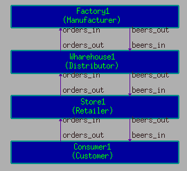
In CSIM, an agent model is used to represent each participant. Each agent has only local information. Agents do not sense the the demand, back-orders, or inventories of other agents. Communication is accomplished only through the placement of orders and receipt of deliveries. The supply-chain diagram of Figure 1 shows the path of orders and shipments.
 |
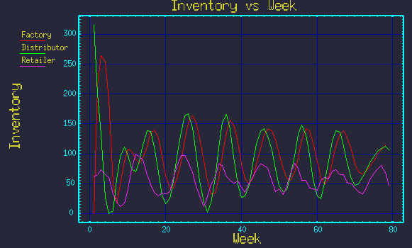
Each players starts with nominally 12 cases (12 beers per case for 144 beers), and initial throughput is 4 cases per week. Figure 2 below shows an example output plot. It is interesting to alter the inventory amounts or supply strategies of the agents to see variations in the resulting dynamics.
 |
Download example model: supplychain.zip
Instructions:
 View Models:
  gui supplychain.sim
  (Or: edit supplychain.sim)

 Build Simulation:
  Tools/ Build Simulation
  (Or:  csim supplychain.sim)

 Run Simulation:
  Tools/Run Simulation
  (Or:  ./sim.exe)

 View Results:
  xgraph factory.dat distributor.dat retailer.dat